This is the third in a five-part series that explores the potential of unified deep learning with CPU, GPU and FGPA technologies. This post discusses DNN implementation, optimization and challenges.
Download the full report.
DNN Implementation and Optimization
Training makes heavy use of floating-point operations for most applications, but for inference operations many network weights can be represented with considerably less precision than their original training output. Recent results show very good results at 8 bits of precision, and in some cases even binary networks can give desired accuracy.
In cases where network weights are zero or near zero, they can be eliminated, or “pruned,” from the graph. Static reduction of weights can account for a modest reduction in weights, while dynamic pruning (done during the inference operation) can achieve considerably higher levels of pruning. Such pruning can considerably reduce the computation requirements for inference operations.
Once a model for deep learning is trained, deploying it for inference in deep learning applications typically has additional requirements. While the compute demand for inference is less in terms of complexity, training data, and long training times, there are several key requirements for inference. In cloud and server systems, inference requirements fall into two categories: low latency single batch, and very large batch high throughput. Inference solutions focus on efficiency of implementation in terms of these requirements. Historically, these tasks have been implemented on CPUs, but GPUs are increasingly being used, and more recently FPGAs have emerged as an efficient solution for inference. FPGAs take advantage of their flexibility to implement lower precision arithmetic, pruned networks, local SRAM, and a wide variety of DRAM standards to provide broad performance, latency, and power envelopes. Inference solutions implemented on FPGAs can be deployed in a datacenter environment as well as in embedded environments like surveillance, self-driving cars, IoT edge servers, etc.
[clickToTweet tweet=”Training makes heavy use of floating-point operations for most applications. #deeplearning” quote=”Training makes heavy use of floating-point operations for most applications. #deeplearning”]
Increasing Computational Challenges
There are a number of standard DNN configurations, each differing by the number of layers and interconnect patterns between layers. The total number of layers has been increasing over time at a rate faster than the “Moore’s Law growth rate” as illustrated in the table below. Between 2012 and 2016, the number of layers in common DNNs have grown by over 2.3x per year. There have been recent discussions of extending the number of layers in future versions of ResNet to 1,000.
DNN training is achieved by fitting the parameters (or weights) using a method called stochastic gradient descent and other optimization techniques to arrive at parameter updates. Iterative updates are required to improve the model accuracy with a small incremental improvement rate. Training with large sample sizes such as ImageNet (containing over 14 million images) and a model such as Resnet can take ~30-40K iterations to converge to a stable solution. As the DNN complexity and the size of the training set both increase, the total computational load, as a high-level estimation, can exceed 1020 FLOPS.
Even with GPU support, it is not unusual for a training session to take days or weeks.
As early as 2008, GPUs were used to speed up the training to an acceptable level. Even with GPU support, it is not unusual for a training session to take days or weeks. There are many optimization strategies being developed to reduce the long learning time. However, as DNNs continue to increase in size and complexity, the computational requirements are expected to grow.
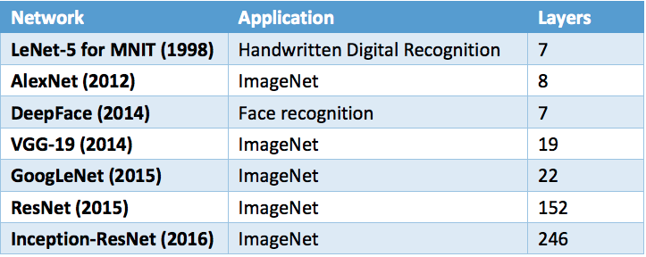
Training Layers Increasing Over Time
In addition to the computational load, the memory capacity and bandwidth are a heavy influence on the overall performance of training, and to a lesser degree, inference. The computation for many network layers has a high compute-to-bandwidth ratio; there is a large amount of data reuse, and the parameters are shared across each layer of input data. Conversely, the more fully connected network layers have very low compute-to-bandwidth ratios; the data reuse is very low and there are no shared parameters.
As GPU processing has improved to address the compute challenges for these networks, many algorithms or models have become bandwidth bound, and the peak performance of the GPU (or CPU) is not realized. In some worst-case conditions the efficiency of the GPU is in the range of 15-20% of peak theoretical performance. This need for increased memory bandwidth being addressed with the use of high bandwidth HBM stacked memory as discussed in the GPU section below.
Over the next few weeks, this series will also cover the following topics:
- The Machine Learning Potential of Combining HPC Technologies
- Exploring the Potential of Deep Learning Software
- Computational Approaches – CPU, GPU, and FPGA
- Unified Deep Learning Configurations and Emerging Applications
You can download the full report here, courtesy of AMD and Xilinx, “Unified Deep Learning with CPU, GPU and FPGA technology.”